

Vector Calculus#
Computing and working with vector calculus on unstructured grids is essential for analyzing scalar and vector fields in geoscience. This notebook demonstrates UXarray’s finite-volume implementations and verifies expected identities.
We will showcase:
Gradient of face-centered scalar fields (zonal and meridional components)
Curl of vector fields (including curl of a gradient ≈ 0 and a synthetic vortex)
Divergence of vector fields (including Laplacian as ∇·∇φ, divergence of a vortex ≈ 0, and radial expansion > 0)
Scalar dot gradient (advection term v · ∇q)
Vector calculus identities verification
Vector calculus for 2D+ arrays (grid dimension plus other dimension(s) such as “time”)
import holoviews as hv
import numpy as np
import xarray as xr

import uxarray as ux

# style: hide DataArray data values by default (click corresponding icon to show)
xr.set_options(display_expand_data=False)

hv.extension("bokeh")

 ⓘ
ⓘ
Data#
This notebook uses a subset of a 30km MPAS atmosphere grid, taken centered at 45 degrees longitude and 0 degrees latitude with a radius of 2 degrees.
face_lon: Longitude at cell-centersface_lat: Latitude at cell-centersgaussian: Gaussian initialized at the center of the gridinverse_gaussian: Inverse of the gaussian above.
uxds = ux.tutorial.open_dataset("mpas-dyamond-30km-gradient")
uxds
<xarray.UxDataset> Size: 3kB
Dimensions:           (n_face: 195)
Dimensions without coordinates: n_face
Data variables:
    face_lat          (n_face) float32 780B ...
    face_lon          (n_face) float32 780B ...
    gaussian          (n_face) float32 780B ...
inverse_gaussian (n_face) float32 780B ...1. Gradient (∇φ)#
Background#
The gradient of a scalar field φ gives both the direction of steepest increase and the rate of change in that direction. On unstructured grids, we use the Green–Gauss theorem:
Implementation#
In a finite-volume context, the gradient of a scalar field \(\phi\) is obtained by summing fluxes across each cell face and dividing by the cell’s volume.
Input |
Usage |
Output |
|---|---|---|
Scalar field \(\phi\) |
|
Vector field \(\nabla\phi\) |
Finite-volume discretization#
Discrete gradient at cell center \(C^*\)#
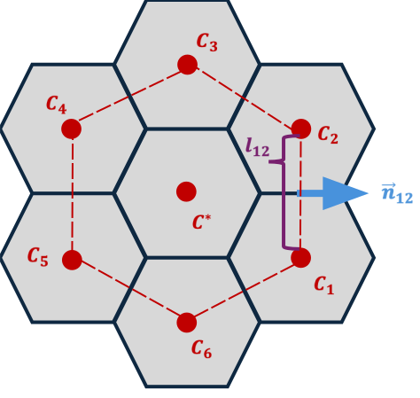
Usage#
Gradients can be computed using the UxDataArray.gradient() method on a face-centered data variable.
Units. By default,
gradient(),curl(), anddivergence()divide byuxgrid.sphere_radiusso derivatives carry physical units (e.g.[data units]/m,1/sfor velocity curl). Passscale_by_radius=Falseto keep results on the unit sphere (per radian). If the grid has nosphere_radiusattribute, the call falls back to unit-sphere output and emits aUserWarning.
grad_lat = uxds["face_lat"].gradient()
grad_lon = uxds["face_lon"].gradient()
grad_gauss = uxds["gaussian"].gradient()
grad_inv_gauss = uxds["inverse_gaussian"].gradient()
Examining one of the outputs, we find that the zonal_gradient and meridional_gradient data variables store the rate of change along longitude (east–west) and latitude (north–south), respectively.
print("Gradient components:")
print(f"Zonal gradient shape: {grad_gauss.zonal_gradient.shape}")
print(f"Meridional gradient shape: {grad_gauss.meridional_gradient.shape}")
grad_gauss
Gradient components:
Zonal gradient shape: (195,)
Meridional gradient shape: (195,)
<xarray.UxDataset> Size: 3kB
Dimensions:              (n_face: 195)
Dimensions without coordinates: n_face
Data variables:
    zonal_gradient       (n_face) float64 2kB nan nan nan nan ... nan nan nan
    meridional_gradient  (n_face) float64 2kB nan nan nan nan ... nan nan nan
Attributes:
gradient: TruePlotting Gradients#
To visualize gradients, we represent them as vector fields and overlay them on the original scalar data.
def plot_gradient_vectors(uxda_grad, **kwargs):
    """
    Plots gradient vectors using HoloViews
    """
    uxgrid = uxda_grad.uxgrid
    mag = np.hypot(uxda_grad.zonal_gradient, uxda_grad.meridional_gradient)
    angle = np.arctan2(uxda_grad.meridional_gradient, uxda_grad.zonal_gradient)

    return hv.VectorField(
        (uxgrid.face_lon, uxgrid.face_lat, angle, mag), **kwargs
    ).opts(magnitude="Magnitude")
# Overlay the gradient vector field on top of the original data variable
p1 = (
    uxds["face_lat"].plot(cmap="Oranges", aspect=1) * plot_gradient_vectors(grad_lat)
).opts(title="∇ Cell Latitudes")
p2 = (
    uxds["face_lon"].plot(cmap="Oranges", aspect=1) * plot_gradient_vectors(grad_lon)
).opts(title="∇ Cell Longitudes")
p3 = (
    uxds["gaussian"].plot(cmap="Oranges", aspect=1) * plot_gradient_vectors(grad_gauss)
).opts(title="∇ Gaussian")
p4 = (
    uxds["inverse_gaussian"].plot(cmap="Oranges", aspect=1)
    * plot_gradient_vectors(grad_inv_gauss)
).opts(title="∇ Inverse Gaussian")

# Compose all four plots in a 2 column layout
(p1 + p2 + p3 + p4).cols(2).opts(shared_axes=False)
2. Curl (∇ × F)#
Background#
The curl of a vector field F = (u, v) measures local rotation. Here \(u\), \(v\) are the zonal and meridional components, \(\lambda\) is longitude, \(\varphi\) is latitude, \(a\) is the sphere radius (uxgrid.sphere_radius), and \(dx = a\cos\varphi\,d\lambda\), \(dy = a\,d\varphi\) are local distances. On a sphere,
The product rule on \(\partial(u\cos\varphi)/\partial\varphi\) produces the last term. It is a metric term: longitude lines converge toward the poles, so a zonal flow rotates even when \(\partial u/\partial y = 0\). It is zero on the equator. In Example 3 it is as large as the derivative term. The NCAR Command Language relative-vorticity documentation gives this full expanded equation and cites Bluestein, Synoptic-Dynamic Meteorology in Midlatitudes (1992), pp. 113–114.
u.curl(v) evaluates the full expression; v.gradient()["zonal_gradient"] - u.gradient()["meridional_gradient"] gives only the first two terms.
Positive curl: Counter-clockwise rotation
Negative curl: Clockwise rotation
Zero curl: No local rotation (irrotational flow)
Usage#
Curl can be computed using the UxDataArray.curl() method on vector field components:
Input |
Usage |
Output |
|---|---|---|
Vector field (u, v) |
|
Scalar curl field |
Constant Fields (Mathematical Validation)#
On a plane the curl of a constant field is zero. On a sphere the derivative terms vanish but the metric term does not, so u.curl(v) \(= u\tan\varphi/a\) exactly.
This subset spans about ±2° of latitude, so \(\tan\varphi/a < 5.5\times10^{-9}\ \mathrm{m^{-1}}\) and the result looks like round-off. It is a real signal; the cell below checks it against \(u\tan\varphi/a\) from the face latitudes.
# Constant vector field: u=1, v=2 (face-centered)
u_constant = uxds["face_lat"] * 0 + 1.0
v_constant = uxds["face_lat"] * 0 + 2.0

curl_constant = u_constant.curl(v_constant)

finite = np.isfinite(curl_constant.values)
vals = curl_constant.values[finite]
print(
    f"Total faces: {curl_constant.size}, interior: {vals.size}, boundary NaNs: {np.isnan(curl_constant.values).sum()}"
)
if vals.size:
    print(f"Finite curl range: [{vals.min():.2e}, {vals.max():.2e}]")
    print(
        f"Max |curl|: {np.abs(vals).max():.2e}, Mean |curl|: {np.abs(vals).mean():.2e}"
    )

# The closed form for a constant u on the sphere is u*tan(lat)/a
lat_rad = np.deg2rad(uxds.uxgrid.face_lat.values)
curl_exact = 1.0 * np.tan(lat_rad) / uxds.uxgrid.sphere_radius
print(f"Max deviation from u*tan(lat)/a: {np.abs(vals - curl_exact[finite]).max():.2e}")
Total faces: 195, interior: 147, boundary NaNs: 48
Finite curl range: [-4.79e-09, 4.59e-09]
Max |curl|: 4.79e-09, Mean |curl|: 2.03e-09
Max deviation from u*tan(lat)/a: 0.00e+00
Gaussian Fields#
# Use Gaussian fields as vector components
u_gauss = uxds["gaussian"]
v_gauss = uxds["inverse_gaussian"]

curl_gauss = u_gauss.curl(v_gauss)

finite = np.isfinite(curl_gauss.values)
vals = curl_gauss.values[finite]
print(
    f"Total faces: {curl_gauss.size}, interior: {vals.size}, boundary NaNs: {np.isnan(curl_gauss.values).sum()}"
)
if vals.size:
    print(f"Finite curl range: [{vals.min():.6e}, {vals.max():.6e}]")
    print(f"Mean curl (finite): {vals.mean():.6e}")
Total faces: 195, interior: 147, boundary NaNs: 48
Finite curl range: [-7.446681e-06, 7.473969e-06]
Mean curl (finite): -1.675887e-08
Example 1: Curl of Gradient Field#
In the continuous setting, curl(∇φ) = 0 exactly for any scalar field φ. On an unstructured mesh, however, gradient and curl are independent finite-volume stencils that do not form a discrete de Rham complex, so the identity holds only approximately. The residual is a discretization error — not a bug — and shrinks with grid refinement.
The magnitude of the residual depends on the units. By default gradient()/curl() scale by uxgrid.sphere_radius (Earth ≈ 6.37×10⁶ m), so each derivative picks up a factor of 1/radius. curl(∇φ) applies the gradient stencil twice and therefore carries a factor of 1/radius² (≈ 2.5×10⁻¹⁴). For the Gaussian field here (φ ~ O(1)) the scaled residual is a few ×10⁻¹⁵; on the unit sphere (scale_by_radius=False) the same residual is ~O(0.1). Either way it shrinks with refinement.
# Extract gradient components and treat them as a vector field
u_component = grad_gauss.zonal_gradient
v_component = grad_gauss.meridional_gradient

curl_of_gradient = u_component.curl(v_component)

print(
    f"Curl of gradient range: [{curl_of_gradient.min().values:.2e}, {curl_of_gradient.max().values:.2e}]"
)
print(f"Mean absolute curl: {abs(curl_of_gradient).mean().values:.2e}")

# Note: values are ~O(1e-15) (per meter^2) with the default radius scaling,
# so we let the color limits autoscale rather than hardcoding them.
curl_plot = curl_of_gradient.plot(cmap="RdBu_r", aspect=1).opts(
    title="Curl of Gradient Field (Should ≈ 0)", colorbar=True
)
curl_plot
Curl of gradient range: [-7.65e-15, 6.61e-15]
Mean absolute curl: 2.76e-15
Example 2: Synthetic Vortex Field#
To better demonstrate curl, let’s create a synthetic rotating vector field (vortex):
# Get face coordinates
face_lon = uxds.uxgrid.face_lon.values
face_lat = uxds.uxgrid.face_lat.values

# Center the coordinates
lon_center = np.mean(face_lon)
lat_center = np.mean(face_lat)

x = face_lon - lon_center
y = face_lat - lat_center

# Create a vortex: u = -y, v = x (pure rotation)
u_vortex_data = -y
v_vortex_data = x

# Create UxDataArrays
u_vortex = ux.UxDataArray(
    u_vortex_data, dims=["n_face"], uxgrid=uxds.uxgrid, name="u_vortex"
)
v_vortex = ux.UxDataArray(
    v_vortex_data, dims=["n_face"], uxgrid=uxds.uxgrid, name="v_vortex"
)

# Compute curl (default: scaled by sphere_radius -> per meter)
curl_vortex = u_vortex.curl(v_vortex)

print(
    f"Vortex curl range: [{curl_vortex.min().values:.2e}, {curl_vortex.max().values:.2e}]"
)
# On the unit sphere this rotation has curl ~2; with the default radius scaling
# the result is that value divided by sphere_radius (positive and roughly uniform).
print(f"Mean vortex curl: {curl_vortex.mean().values:.2e} (positive => rotational)")
Vortex curl range: [1.80e-05, 1.80e-05]
Mean vortex curl: 1.80e-05 (positive => rotational)
# Plot the vortex vector field and its curl
def plot_vector_field(u, v, **kwargs):
    """Plot vector field using HoloViews"""
    uxgrid = u.uxgrid
    mag = np.hypot(u, v)
    angle = np.arctan2(v, u)

    return hv.VectorField(
        (uxgrid.face_lon, uxgrid.face_lat, angle, mag), **kwargs
    ).opts(magnitude="Magnitude")


# Vector field plot
vortex_vectors = plot_vector_field(u_vortex, v_vortex).opts(
    title="Synthetic Vortex Field", aspect=1, arrow_heads=True
)

# Curl magnitude plot
curl_magnitude = curl_vortex.plot(cmap="Reds", aspect=1).opts(
    title="Curl of Vortex Field", colorbar=True
)

(vortex_vectors + curl_magnitude).opts(shared_axes=False)
Example 3: Relative Vorticity from Solid-Body Rotation#
The curl on the sphere is relative vorticity \(\zeta\): the local spinning motion of the flow relative to Earth’s surface. With the default scale_by_radius=True, u.curl(v) returns \(\zeta\) in \(s^{-1}\).
A clean analytical check is solid-body rotation about the polar axis, in which every point circles the axis with the same angular speed \(\Omega\). Here \(R\) is Earth’s radius, \(\varphi\) is latitude, and \(u\) and \(v\) are the eastward and northward speeds. The eastward speed decreases toward the poles because a point there traces a smaller circle:
The result is the planetary vorticity \(f\), the local vertical component of the rotation associated with Earth. The derivative term and the metric term each contribute \(\Omega\sin\varphi\), so a flat-plane formula, which omits the sphere’s curvature, would return half the answer. We compare u.curl(v) against \(2\Omega\sin\varphi\) on the MPAS subset.
OMEGA = 7.292115e-5  # Earth's angular speed (rad/s)
R = uxds.uxgrid.sphere_radius
lat_rad = np.deg2rad(uxds.uxgrid.face_lat.values)

u_sbr_data = OMEGA * R * np.cos(lat_rad)
v_sbr_data = np.zeros_like(u_sbr_data)

u_sbr = ux.UxDataArray(
    u_sbr_data,
    dims=["n_face"],
    uxgrid=uxds.uxgrid,
    name="u_sbr",
    attrs={"units": "m/s"},
)
v_sbr = ux.UxDataArray(
    v_sbr_data,
    dims=["n_face"],
    uxgrid=uxds.uxgrid,
    name="v_sbr",
    attrs={"units": "m/s"},
)

zeta = u_sbr.curl(v_sbr)
zeta_analytic = 2.0 * OMEGA * np.sin(lat_rad)

finite = np.isfinite(zeta.values)
err = np.abs(zeta.values[finite] - zeta_analytic[finite])

print(f"curl units: {zeta.attrs['units']}")
print(f"sphere_radius (m): {R:.3e}")
print(
    f"computed   zeta range: [{zeta.values[finite].min():.3e}, {zeta.values[finite].max():.3e}]  1/s"
)
print(
    f"analytic   zeta range: [{zeta_analytic[finite].min():.3e}, {zeta_analytic[finite].max():.3e}]  1/s"
)
print(
    f"max |error|: {err.max():.3e}  1/s  (≈ {err.max() / np.abs(zeta_analytic[finite]).max():.2%} of max |zeta|)"
)
curl units: (m/s)/m
sphere_radius (m): 6.371e+06
computed   zeta range: [-4.448e-06, 4.259e-06]  1/s
analytic   zeta range: [-4.447e-06, 4.259e-06]  1/s
max |error|: 8.523e-10  1/s  (≈ 0.02% of max |zeta|)
zeta.plot(cmap="RdBu_r", aspect=1).opts(
    title="Relative Vorticity (1/s) — Solid-Body Rotation", colorbar=True
)
3. Divergence (∇ · F)#
Background#
The divergence of a vector field F = (u, v) measures the local expansion or contraction of the field. It carries the companion of the metric term in curl, with the opposite sign and the meridional component in place of the zonal one:
Positive divergence: Expansion (source)
Negative divergence: Contraction (sink)
Zero divergence: Incompressible flow
Usage#
Divergence can be computed using the UxDataArray.divergence() method:
Input |
Usage |
Output |
|---|---|---|
Vector field (u, v) |
|
Scalar divergence field |
Constant Fields (Mathematical Validation)#
As with curl, a constant field is divergence-free on a plane but not on a sphere. The derivative terms vanish and the metric term leaves \(-v\tan\varphi/a\), which is twice the curl residual above and of the opposite sign, since \(v = 2u\) here.
# Constant vector field: u=1, v=2 (face-centered)
u_constant = uxds["face_lat"] * 0 + 1.0
v_constant = uxds["face_lat"] * 0 + 2.0

div_constant = u_constant.divergence(v_constant)

finite = np.isfinite(div_constant.values)
vals = div_constant.values[finite]
print(
    f"Total faces: {div_constant.size}, interior: {vals.size}, boundary NaNs: {np.isnan(div_constant.values).sum()}"
)
if vals.size:
    print(f"Finite divergence range: [{vals.min():.2e}, {vals.max():.2e}]")
    print(f"Max |div|: {np.abs(vals).max():.2e}, Mean |div|: {np.abs(vals).mean():.2e}")

# The closed form for a constant v on the sphere is -v*tan(lat)/a
div_exact = -2.0 * np.tan(lat_rad) / uxds.uxgrid.sphere_radius
print(f"Max deviation from -v*tan(lat)/a: {np.abs(vals - div_exact[finite]).max():.2e}")
Total faces: 195, interior: 147, boundary NaNs: 48
Finite divergence range: [-9.17e-09, 9.58e-09]
Max |div|: 9.58e-09, Mean |div|: 4.06e-09
Max deviation from -v*tan(lat)/a: 0.00e+00
Gaussian Fields#
# Use Gaussian fields as vector components
u_gauss = uxds["gaussian"]
v_gauss = uxds["inverse_gaussian"]

div_gauss = u_gauss.divergence(v_gauss)

finite = np.isfinite(div_gauss.values)
vals = div_gauss.values[finite]
print(
    f"Total faces: {div_gauss.size}, interior: {vals.size}, boundary NaNs: {np.isnan(div_gauss.values).sum()}"
)
if vals.size:
    print(f"Finite divergence range: [{vals.min():.6e}, {vals.max():.6e}]")
    print(f"Mean divergence (finite): {vals.mean():.6e}")
Total faces: 195, interior: 147, boundary NaNs: 48
Finite divergence range: [-7.407602e-06, 7.497185e-06]
Mean divergence (finite): 5.094522e-08
Example 1: Divergence of Gradient Field#
# Compute divergence of the gradient (Laplacian)
# ∇²φ = ∂(∇φ_x)/∂x + ∂(∇φ_y)/∂y
grad_gauss_u = grad_gauss["zonal_gradient"]
grad_gauss_v = grad_gauss["meridional_gradient"]

div_of_gradient = grad_gauss_u.divergence(grad_gauss_v)

print(
    f"Divergence of gradient range: [{div_of_gradient.min().values:.2e}, {div_of_gradient.max().values:.2e}]"
)
print("This is the Laplacian (∇²) of the original gaussian field")

div_plot = div_of_gradient.plot(cmap="RdBu_r", aspect=1).opts(
    title="Divergence of Gradient (Laplacian)", colorbar=True
)
div_plot
Divergence of gradient range: [-1.49e-10, 2.82e-12]
This is the Laplacian (∇²) of the original gaussian field
Example 2: Divergence of Vortex Field#
Pure rotation is incompressible, so the divergence should be ≈ 0. The metric term \(-v\tan\varphi/a\) is not identically zero here, so the residual (~4×10⁻⁹) is an order of magnitude above the derivative terms alone (~3×10⁻¹⁰) and four orders below the ~10⁻⁵ signal in the radial case below.
div_vortex = u_vortex.divergence(v_vortex)

print(
    f"Vortex divergence range: [{div_vortex.min().values:.2e}, {div_vortex.max().values:.2e}]"
)
print(f"Mean absolute divergence: {abs(div_vortex).mean().values:.2e}")
print("Pure rotation should have zero divergence")

# Residual is ~O(1e-9) with default radius scaling; let color limits autoscale.
div_vortex_plot = div_vortex.plot(cmap="RdBu_r", aspect=1).opts(
    title="Divergence of Vortex (Should ≈ 0)", colorbar=True
)
div_vortex_plot
Vortex divergence range: [-3.72e-09, 4.00e-09]
Mean absolute divergence: 1.31e-09
Pure rotation should have zero divergence
Example 3: Radial Expansion Field#
Let’s create a field that expands radially outward to demonstrate positive divergence:
# Create radial expansion field: u = x, v = y
u_radial_data = x
v_radial_data = y

u_radial = ux.UxDataArray(
    u_radial_data, dims=["n_face"], uxgrid=uxds.uxgrid, name="u_radial"
)
v_radial = ux.UxDataArray(
    v_radial_data, dims=["n_face"], uxgrid=uxds.uxgrid, name="v_radial"
)

# Compute curl and divergence (default: scaled by sphere_radius)
curl_radial = u_radial.curl(v_radial)
div_radial = u_radial.divergence(v_radial)

print(
    f"Radial field curl range: [{curl_radial.min().values:.2e}, {curl_radial.max().values:.2e}]"
)
print(
    f"Radial field divergence range: [{div_radial.min().values:.2e}, {div_radial.max().values:.2e}]"
)
# On the unit sphere this expansion has curl ~0 and divergence ~2; with the
# default radius scaling both are divided by sphere_radius.
print(
    "Expected (unit sphere): curl ≈ 0, divergence ≈ 2; scaled values are /radius smaller"
)
Radial field curl range: [-4.00e-09, 3.72e-09]
Radial field divergence range: [1.80e-05, 1.80e-05]
Expected (unit sphere): curl ≈ 0, divergence ≈ 2; scaled values are /radius smaller
# Plot radial expansion field and its divergence
radial_vectors = plot_vector_field(u_radial, v_radial).opts(
    title="Radial Expansion Field", aspect=1, arrow_heads=True
)

radial_div = div_radial.plot(cmap="Reds", aspect=1).opts(
    title="Divergence of Radial Field", colorbar=True
)

(radial_vectors + radial_div).opts(shared_axes=False)
4. Scalar Dot Gradient (v · ∇q)#
Background#
Many geophysical applications need the projection of a vector field v = (u, v) onto the gradient of a scalar field q. This quantity appears, for example, as the horizontal advection term in transport equations:
Usage#
The UxDataArray.scalardotgradient(v, q) method computes this dot product directly. The data variable it is called on (self) is treated as the zonal component u, v is the meridional component, and q is the scalar field whose gradient is taken. All three inputs must be face-centered and share the same grid and dimensions.
# Treat the Gaussian and its inverse as a vector field (u, v)
u_field = uxds["gaussian"]
v_field = uxds["inverse_gaussian"]

# Scalar field whose gradient is advected
q_field = uxds["gaussian"]

# v . grad(q) = u * dq/dx + v * dq/dy
vdotgradq = u_field.scalardotgradient(v_field, q_field)
vdotgradq
<xarray.UxDataArray 'scalardotgradient_gaussian_inverse_gaussian_gaussian' (
                                                                            n_face: 195)> Size: 2kB
nan nan nan nan 1.877e-06 nan 2.27e-06 ... nan -2.692e-06 nan nan nan nan
Dimensions without coordinates: n_face
Attributes:
    units:              1/m
    long_name:          Scalar dot gradient: (gaussian, inverse_gaussian) dot...
    scalardotgradient:  True
description: Dot product of vector field (u, v) with the gradient ...# Verify against an explicit gradient-based computation
grad_q = q_field.gradient()
expected = u_field * grad_q["zonal_gradient"] + v_field * grad_q["meridional_gradient"]
# Boundary faces yield NaN gradients, so compare only finite values
finite = np.isfinite(vdotgradq.values) & np.isfinite(expected.values)
max_diff = np.abs(vdotgradq.values[finite] - expected.values[finite]).max()
print(f"Max difference vs. explicit u*dq/dx + v*dq/dy: {max_diff:.2e}")
print(f"Matches explicit computation: {max_diff < 1e-12}")
Max difference vs. explicit u*dq/dx + v*dq/dy: 0.00e+00
Matches explicit computation: True
# Visualize the scalar dot gradient field
vdotgradq.plot(cmap="RdBu_r", aspect=1).opts(
    title="Scalar Dot Gradient  v · ∇q", colorbar=True
)
5. Vector Calculus Identities#
Let’s verify some fundamental vector calculus identities using our computed fields:
Identity 1: Curl of Gradient (Discretization Residual)#
In the continuous setting: ∇ × (∇φ) = 0. UXarray’s finite-volume operators are not mimetic, so this holds only approximately. The residual below is discretization error, not a numerical bug. With the default radius scaling it is a few ×10⁻¹⁵ for this φ ~ O(1) field (the curl stencil applies a 1/radius² factor); on the unit sphere it is ~O(0.1). It shrinks with grid refinement.
# We already computed this above
max_curl_grad = np.abs(curl_of_gradient).max().values
print(f"Maximum |curl(∇φ)|: {max_curl_grad:.2e}")
print(
    "Note: non-zero residual is expected discretization error from independent "
    "finite-volume gradient and curl stencils (not a bug). Shrinks with grid refinement."
)
Maximum |curl(∇φ)|: 7.65e-15
Note: non-zero residual is expected discretization error from independent finite-volume gradient and curl stencils (not a bug). Shrinks with grid refinement.
Identity 2: Divergence of Curl is Zero#
For any vector field F: ∇ · (∇ × F) = 0
Note: This identity applies to 3D vector fields. In 2D, curl produces a scalar, so we can’t directly compute its divergence.
Identity 3: Properties of Special Fields#
# Summary of field properties
print("Field Properties Summary:")
print("=" * 50)
print("Gradient field:")
print(f"  - Curl: {np.abs(curl_of_gradient).max().values:.2e} (≈ 0, conservative)")
print(
    f"  - Divergence: {div_of_gradient.min().values:.2e} to {div_of_gradient.max().values:.2e} (Laplacian)"
)
print()
print("Vortex field (pure rotation):")
print(f"  - Curl: {curl_vortex.mean().values:.2e} (> 0, rotational)")
print(f"  - Divergence: {np.abs(div_vortex).max().values:.2e} (≈ 0, incompressible)")
print()
print("Radial field (pure expansion):")
print(f"  - Curl: {np.abs(curl_radial).max().values:.2e} (≈ 0, irrotational)")
print(f"  - Divergence: {div_radial.mean().values:.2e} (> 0, expanding)")
Field Properties Summary:
==================================================
Gradient field:
  - Curl: 7.65e-15 (≈ 0, conservative)
  - Divergence: -1.49e-10 to 2.82e-12 (Laplacian)

Vortex field (pure rotation):
  - Curl: 1.80e-05 (> 0, rotational)
  - Divergence: 4.00e-09 (≈ 0, incompressible)

Radial field (pure expansion):
  - Curl: 4.00e-09 (≈ 0, irrotational)
  - Divergence: 1.80e-05 (> 0, expanding)
6. Vector calculus for 2D+ arrays#
Real data often has multiple dimensions such as “time” or “levels”, not just the grid dimension.
In uxarray, vector calculus operators simply loop across other dimensions in the intuitive way. For example, for an array with “time” and “n_face”, applying .gradient() will take the gradient at each point in time, then join results along the “time” dimension.
CAUTION: the default “scale result by grid radius” behavior does not automatically account for any radius differences across vertical levels in the data, it simply divides by the radius of the grid.
Example: time-varying vortex#
Let’s add some time variation to the vortex example from above.
# Make up some time variation
t = [0, 0.25, 0.75, 1.0]  # pick some times
times = xr.DataArray(t, dims="time", coords={"time": t})
variation = np.cos(np.pi * times)

u_vary = (u_vortex * variation).rename("u_varying")
v_vary = (v_vortex * variation).rename("v_varying")
variation
<xarray.DataArray (time: 4)> Size: 32B
1.0 0.7071 -0.7071 -1.0
Coordinates:
  * time     (time) float64 32B 0.0 0.25 0.75 1.0
# Plot the underlying data
ncols = 2

panels = []
for i in range(len(times)):
    arrows = plot_vector_field(u_vary.isel(time=i), v_vary.isel(time=i)).opts(
        title=f"Synthetic vortex at t={times.isel(time=i):.2f}"
    )
    panels.append(arrows)

hv.Layout(panels).cols(ncols)
# Take the curl
curl = u_vary.curl(v_vary)
curl
<xarray.UxDataArray 'curl_u_varying_v_varying' (n_face: 195, time: 4)> Size: 6kB
nan nan nan nan nan nan nan nan nan nan ... nan nan nan nan nan nan nan nan nan
Coordinates:
  * time     (time) float64 32B 0.0 0.25 0.75 1.0
Dimensions without coordinates: n_face
Attributes:
    units:        1/m
    long_name:    Curl of (u_varying, v_varying)
    curl:         True
description: Curl of vector field computed as ∂v/∂x - ∂u/∂y + u·tan(φ)/a...# Check: is it equivalent to taking curl at each point in time?
curl_from_slices = ux.concat(
[u_vary.isel(time=i).curl(v_vary.isel(time=i)) for i in range(len(times))],
dim="time",
)
# Confirm the values are the same; the difference is always 0
# (Can't use np.allclose directly, due to NaN values; (NaN == NaN) is False.)
diff = curl_from_slices - curl
print("(min, max) of curl_from_slices - curl: ", (diff.min().item(), diff.max().item()))
(min, max) of curl_from_slices - curl: (0.0, 0.0)
# Plot the curl, with arrows overlayed:
ncols = 2

curl_vmax = np.abs(curl).max().item()

panels = []
for i in range(len(times)):
    shading = curl.isel(time=i).plot(
        cmap="RdBu_r",
        clim=(-curl_vmax, curl_vmax),
        colorbar=(i % ncols == ncols - 1),  # colorbars only on rightmost plots
        title=f"Curl at t={t[i]:.2f}",
        aspect=1,
    )
    arrows = plot_vector_field(u_vary.isel(time=i), v_vary.isel(time=i))
    panels.append(shading * arrows)

hv.Layout(panels).cols(ncols)
# It is also possible to plot as a single animation in time, instead:
curl_vmax = np.abs(curl).max().item()


def frame(i):
    shading = curl.isel(time=i).plot(
        cmap="RdBu_r",
        clim=(-curl_vmax, curl_vmax),
        colorbar=True,
        aspect=1,
    )
    arrows = plot_vector_field(u_vary.isel(time=i), v_vary.isel(time=i))
    return shading * arrows


anim = hv.HoloMap(
    {f"Curl at t={t[i]:.2f}": frame(i) for i in range(len(times))}, kdims="time"
)
hv.output(holomap="scrubber", fps=1)
anim